Cite From: https://towardsdatascience.com/how-to-code-the-transformer-in-pytorch-24db27c8f9ec

 

Could The Transformer be another nail in the coffin for RNNs?

Doing away with the clunky for loops, it finds a way to allow whole sentences to simultaneously enter the network in batches. The miracle; NLP now reclaims the advantage of python’s highly efficient linear algebra libraries. This time-saving can then spent deploying more layers into the model.

So far it seems the result is faster convergence and better results. What’s not to love?

My personal experience of it has been highly promising. It trained on 2 million French-English sentence pairs to create a sophisticated translator in only three days.

You can play with the model yourself on language translating tasks if you go to my implementation on Github here. Also check out my next post, where I share my journey building the translator and the results.

Or finally, you could build one yourself. Here’s the guide on how to do it, and how it works.

This guide only explains how to code the model and run it, for information on how to obtain data and process it for seq2seq see my guide here.

The Transformer

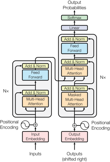
The diagram above shows the overview of the Transformer model. The inputs to the encoder will be the English sentence, and the ‘Outputs‘ entering the decoder will be the French sentence.

In effect, there are five processes we need to understand to implement this model:

• Embedding the inputs
• The Positional Encodings
• Creating Masks
• The Multi-Head Attention layer
• The Feed-Forward layer

Embedding

Embedding words has become standard practice in NMT, feeding the network with far more information about words than a one hot encoding would. For more information on this see my post here.

Embedding is handled simply in pytorch:

class Embedder(nn.Module):
    def __init__(self, vocab_size, d_model):
        super().__init__()
        self.embed = nn.Embedding(vocab_size, d_model)
    def forward(self, x):
        return self.embed(x)

When each word is fed into the network, this code will perform a look-up and retrieve its embedding vector. These vectors will then be learnt as a parameters by the model, adjusted with each iteration of gradient descent.

Giving our words context: The positional encoding

In order for the model to make sense of a sentence, it needs to know two things about each word: what does the word mean? And what is its position in the sentence?

The embedding vector for each word will learn the meaning, so now we need to input something that tells the network about the word’s position.

Vasmari et al answered this problem by using these functions to create a constant of position-specific values:

This constant is a 2d matrix. Pos refers to the order in the sentence, and i refers to the position along the embedding vector dimension. Each value in the pos/i matrix is then worked out using the equations above.

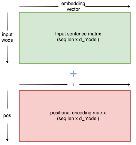
An intuitive way of coding our Positional Encoder looks like this:

class PositionalEncoder(nn.Module):
    def __init__(self, d_model, max_seq_len = 80):
        super().__init__()
        self.d_model = d_model
        
        # create constant 'pe' matrix with values dependant on 
        # pos and i
        pe = torch.zeros(max_seq_len, d_model)
        for pos in range(max_seq_len):
            for i in range(0, d_model, 2):
                pe[pos, i] = \
                math.sin(pos / (10000 ** ((2 * i)/d_model)))
                pe[pos, i + 1] = \
                math.cos(pos / (10000 ** ((2 * (i + 1))/d_model)))
                
        pe = pe.unsqueeze(0)
        self.register_buffer('pe', pe)
 
    
    def forward(self, x):
        # make embeddings relatively larger
        x = x * math.sqrt(self.d_model)
        #add constant to embedding
        seq_len = x.size(1)
        x = x + Variable(self.pe[:,:seq_len], \
        requires_grad=False).cuda()
        return x

The above module lets us add the positional encoding to the embedding vector, providing information about structure to the model.

The reason we increase the embedding values before addition is to make the positional encoding relatively smaller. This means the original meaning in the embedding vector won’t be lost when we add them together.

Creating Our Masks

Masking plays an important role in the transformer. It serves two purposes:

• In the encoder and decoder: To zero attention outputs wherever there is just padding in the input sentences.
• In the decoder: To prevent the decoder ‘peaking’ ahead at the rest of the translated sentence when predicting the next word.

Creating the mask for the input is simple:

batch = next(iter(train_iter))
input_seq = batch.English.transpose(0,1)
input_pad = EN_TEXT.vocab.stoi['<pad>']# creates mask with 0s wherever there is padding in the input
input_msk = (input_seq != input_pad).unsqueeze(1)

For the target_seq we do the same, but then create an additional step:

# create mask as beforetarget_seq = batch.French.transpose(0,1)
target_pad = FR_TEXT.vocab.stoi['<pad>']
target_msk = (target_seq != target_pad).unsqueeze(1)size = target_seq.size(1) # get seq_len for matrixnopeak_mask = np.triu(np.ones(1, size, size),
k=1).astype('uint8')
nopeak_mask = Variable(torch.from_numpy(nopeak_mask) == 0)target_msk = target_msk & nopeak_mask

The initial input into the decoder will be the target sequence (the French translation). The way the decoder predicts each output word is by making use of all the encoder outputs and the French sentence only up until the point of each word its predicting.

Therefore we need to prevent the first output predictions from being able to see later into the sentence. For this we use the nopeak_mask:

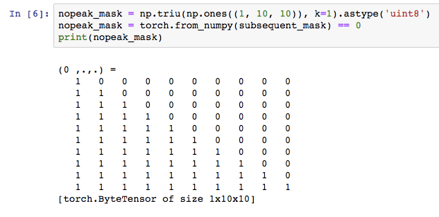
If we later apply this mask to the attention scores, the values wherever the input is ahead will not be able to contribute when calculating the outputs.

Multi-Headed Attention

Once we have our embedded values (with positional encodings) and our masks, we can start building the layers of our model.

Here is an overview of the multi-headed attention layer:

V, K and Q stand for ‘key’, ‘value’ and ‘query’. These are terms used in attention functions, but honestly, I don’t think explaining this terminology is particularly important for understanding the model.

In the case of the Encoder, V, K and G will simply be identical copies of the embedding vector (plus positional encoding). They will have the dimensions Batch_size * seq_len * d_model.

In multi-head attention we split the embedding vector into N heads, so they will then have the dimensions batch_size * N * seq_len * (d_model / N).

This final dimension (d_model / N ) we will refer to as d_k.

Let’s see the code for the decoder module:

class MultiHeadAttention(nn.Module):
    def __init__(self, heads, d_model, dropout = 0.1):
        super().__init__()
        
        self.d_model = d_model
        self.d_k = d_model // heads
        self.h = heads
        
        self.q_linear = nn.Linear(d_model, d_model)
        self.v_linear = nn.Linear(d_model, d_model)
        self.k_linear = nn.Linear(d_model, d_model)
        self.dropout = nn.Dropout(dropout)
        self.out = nn.Linear(d_model, d_model)
    
    def forward(self, q, k, v, mask=None):
        
        bs = q.size(0)
        
        # perform linear operation and split into h heads
        
        k = self.k_linear(k).view(bs, -1, self.h, self.d_k)
        q = self.q_linear(q).view(bs, -1, self.h, self.d_k)
        v = self.v_linear(v).view(bs, -1, self.h, self.d_k)
        
        # transpose to get dimensions bs * h * sl * d_model
       
        k = k.transpose(1,2)
        q = q.transpose(1,2)
        v = v.transpose(1,2)# calculate attention using function we will define next
        scores = attention(q, k, v, self.d_k, mask, self.dropout)
        
        # concatenate heads and put through final linear layer
        concat = scores.transpose(1,2).contiguous()\
        .view(bs, -1, self.d_model)
        
        output = self.out(concat)
    
        return output

Calculating Attention

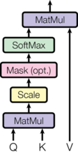
This is the only other equation we will be considering today, and this diagram from the paper does a god job at explaining each step.

Each arrow in the diagram reflects a part of the equation.

Initially we must multiply Q by the transpose of K. This is then ‘scaled’ by dividing the output by the square root of d_k.

A step that’s not shown in the equation is the masking operation. Before we perform Softmax, we apply our mask and hence reduce values where the input is padding (or in the decoder, also where the input is ahead of the current word).

Another step not shown is dropout, which we will apply after Softmax.

Finally, the last step is doing a dot product between the result so far and V.

Here is the code for the attention function:

def attention(q, k, v, d_k, mask=None, dropout=None):
    
    scores = torch.matmul(q, k.transpose(-2, -1)) /  math.sqrt(d_k)if mask is not None:
        mask = mask.unsqueeze(1)
        scores = scores.masked_fill(mask == 0, -1e9)scores = F.softmax(scores, dim=-1)
    
    if dropout is not None:
        scores = dropout(scores)
        
    output = torch.matmul(scores, v)
    return output

The Feed-Forward Network

Ok if you’ve understood so far, give yourself a big pat on the back as we’ve made it to the final layer and it’s all pretty simple from here!

This layer just consists of two linear operations, with a relu and dropout operation in between them.

class FeedForward(nn.Module):
    def __init__(self, d_model, d_ff=2048, dropout = 0.1):
        super().__init__() 
        # We set d_ff as a default to 2048
        self.linear_1 = nn.Linear(d_model, d_ff)
        self.dropout = nn.Dropout(dropout)
        self.linear_2 = nn.Linear(d_ff, d_model)
    def forward(self, x):
        x = self.dropout(F.relu(self.linear_1(x)))
        x = self.linear_2(x)
        return x

The feed-forward layer simply deepens our network, employing linear layers to analyse patterns in the attention layers output.

One Last Thing : Normalisation

Normalisation is highly important in deep neural networks. It prevents the range of values in the layers changing too much, meaning the model trains faster and has better ability to generalise.

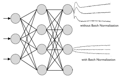
We will be normalising our results between each layer in the encoder/decoder, so before building our model let’s define that function:

class Norm(nn.Module):
    def __init__(self, d_model, eps = 1e-6):
        super().__init__()
    
        self.size = d_model
        # create two learnable parameters to calibrate normalisation
        self.alpha = nn.Parameter(torch.ones(self.size))
        self.bias = nn.Parameter(torch.zeros(self.size))
        self.eps = eps
    def forward(self, x):
        norm = self.alpha * (x - x.mean(dim=-1, keepdim=True)) \
        / (x.std(dim=-1, keepdim=True) + self.eps) + self.bias
        return norm

Putting it all together!

If you understand the details above, you now understand the model. The rest is simply putting everything into place.

Let’s have another look at the over-all architecture and start building:

One last Variable: If you look at the diagram closely you can see a ‘Nx’ next to the encoder and decoder architectures. In reality, the encoder and decoder in the diagram above represent one layer of an encoder and one of the decoder. N is the variable for the number of layers there will be. Eg. if N=6, the data goes through six encoder layers (with the architecture seen above), then these outputs are passed to the decoder which also consists of six repeating decoder layers.

We will now build EncoderLayer and DecoderLayer modules with the architecture shown in the model above. Then when we build the encoder and decoder we can define how many of these layers to have.

# build an encoder layer with one multi-head attention layer and one # feed-forward layerclass EncoderLayer(nn.Module):
    def __init__(self, d_model, heads, dropout = 0.1):
        super().__init__()
        self.norm_1 = Norm(d_model)
        self.norm_2 = Norm(d_model)
        self.attn = MultiHeadAttention(heads, d_model)
        self.ff = FeedForward(d_model)
        self.dropout_1 = nn.Dropout(dropout)
        self.dropout_2 = nn.Dropout(dropout)
        
    def forward(self, x, mask):
        x2 = self.norm_1(x)
        x = x + self.dropout_1(self.attn(x2,x2,x2,mask))
        x2 = self.norm_2(x)
        x = x + self.dropout_2(self.ff(x2))
        return x
    
# build a decoder layer with two multi-head attention layers and
# one feed-forward layerclass DecoderLayer(nn.Module):
    def __init__(self, d_model, heads, dropout=0.1):
        super().__init__()
        self.norm_1 = Norm(d_model)
        self.norm_2 = Norm(d_model)
        self.norm_3 = Norm(d_model)
        
        self.dropout_1 = nn.Dropout(dropout)
        self.dropout_2 = nn.Dropout(dropout)
        self.dropout_3 = nn.Dropout(dropout)
        
        self.attn_1 = MultiHeadAttention(heads, d_model)
        self.attn_2 = MultiHeadAttention(heads, d_model)
        self.ff = FeedForward(d_model).cuda()def forward(self, x, e_outputs, src_mask, trg_mask):
        x2 = self.norm_1(x)
        x = x + self.dropout_1(self.attn_1(x2, x2, x2, trg_mask))
        x2 = self.norm_2(x)
        x = x + self.dropout_2(self.attn_2(x2, e_outputs, e_outputs,
        src_mask))
        x2 = self.norm_3(x)
        x = x + self.dropout_3(self.ff(x2))
        return x# We can then build a convenient cloning function that can generate multiple layers:def get_clones(module, N):
    return nn.ModuleList([copy.deepcopy(module) for i in range(N)])

We’re now ready to build the encoder and decoder:

class Encoder(nn.Module):
    def __init__(self, vocab_size, d_model, N, heads):
        super().__init__()
        self.N = N
        self.embed = Embedder(vocab_size, d_model)
        self.pe = PositionalEncoder(d_model)
        self.layers = get_clones(EncoderLayer(d_model, heads), N)
        self.norm = Norm(d_model)
    def forward(self, src, mask):
        x = self.embed(src)
        x = self.pe(x)
        for i in range(N):
            x = self.layers[i](x, mask)
        return self.norm(x)
    
class Decoder(nn.Module):
    def __init__(self, vocab_size, d_model, N, heads):
        super().__init__()
        self.N = N
        self.embed = Embedder(vocab_size, d_model)
        self.pe = PositionalEncoder(d_model)
        self.layers = get_clones(DecoderLayer(d_model, heads), N)
        self.norm = Norm(d_model)
    def forward(self, trg, e_outputs, src_mask, trg_mask):
        x = self.embed(trg)
        x = self.pe(x)
        for i in range(self.N):
            x = self.layers[i](x, e_outputs, src_mask, trg_mask)
        return self.norm(x)

And finally… The transformer!

class Transformer(nn.Module):
    def __init__(self, src_vocab, trg_vocab, d_model, N, heads):
        super().__init__()
        self.encoder = Encoder(src_vocab, d_model, N, heads)
        self.decoder = Decoder(trg_vocab, d_model, N, heads)
        self.out = nn.Linear(d_model, trg_vocab)
    def forward(self, src, trg, src_mask, trg_mask):
        e_outputs = self.encoder(src, src_mask)
        d_output = self.decoder(trg, e_outputs, src_mask, trg_mask)
        output = self.out(d_output)
        return output# we don't perform softmax on the output as this will be handled 
# automatically by our loss function

Training the model

With the transformer built, all that remains is to train that sucker on the EuroParl dataset. The coding part is pretty painless, but be prepared to wait for about 2 days for this model to start converging!

Let’s define some parameters first:

d_model = 512
heads = 8
N = 6
src_vocab = len(EN_TEXT.vocab)
trg_vocab = len(FR_TEXT.vocab)model = Transformer(src_vocab, trg_vocab, d_model, N, heads)for p in model.parameters():
    if p.dim() > 1:
        nn.init.xavier_uniform_(p)# this code is very important! It initialises the parameters with a
# range of values that stops the signal fading or getting too big.
# See this blog for a mathematical explanation.optim = torch.optim.Adam(model.parameters(), lr=0.0001, betas=(0.9, 0.98), eps=1e-9)

And now we’re good to train:

def train_model(epochs, print_every=100):
    
    model.train()
    
    start = time.time()
    temp = start
    
    total_loss = 0
    
    for epoch in range(epochs):
       
        for i, batch in enumerate(train_iter):            src = batch.English.transpose(0,1)
            trg = batch.French.transpose(0,1)            # the French sentence we input has all words except
            # the last, as it is using each word to predict the next
            
            trg_input = trg[:, :-1]
            
            # the words we are trying to predict
            
            targets = trg[:, 1:].contiguous().view(-1)
            
            # create function to make masks using mask code above
            
            src_mask, trg_mask = create_masks(src, trg_input)
            
            preds = model(src, trg_input, src_mask, trg_mask)
            
            optim.zero_grad()
            
            loss = F.cross_entropy(preds.view(-1, preds.size(-1)),
            results, ignore_index=target_pad)            loss.backward()
            optim.step()
            
            total_loss += loss.data[0]
            if (i + 1) % print_every == 0:
                loss_avg = total_loss / print_every
                print("time = %dm, epoch %d, iter = %d, loss = %.3f,
                %ds per %d iters" % ((time.time() - start) // 60,
                epoch + 1, i + 1, loss_avg, time.time() - temp,
                print_every))
                total_loss = 0
                temp = time.time()

Testing the model

We can use the below function to translate sentences. We can feed it sentences directly from our batches, or input custom strings.

The translator works by running a loop. We start off by encoding the English sentence. We then feed the decoder the <sos> token index and the encoder outputs. The decoder makes a prediction for the first word, and we add this to our decoder input with the sos token. We rerun the loop, getting the next prediction and adding this to the decoder input, until we reach the <eos> token letting us know it has finished translating.

def translate(model, src, max_len = 80, custom_string=False):
    
    model.eval()if custom_sentence == True:
        src = tokenize_en(src)
        sentence=\
        Variable(torch.LongTensor([[EN_TEXT.vocab.stoi[tok] for tok
        in sentence]])).cuda()src_mask = (src != input_pad).unsqueeze(-2)
    e_outputs = model.encoder(src, src_mask)
    
    outputs = torch.zeros(max_len).type_as(src.data)
    outputs[0] = torch.LongTensor([FR_TEXT.vocab.stoi['<sos>']])for i in range(1, max_len):    
            
        trg_mask = np.triu(np.ones((1, i, i),
        k=1).astype('uint8')
        trg_mask= Variable(torch.from_numpy(trg_mask) == 0).cuda()
        
        out = model.out(model.decoder(outputs[:i].unsqueeze(0),
        e_outputs, src_mask, trg_mask))
        out = F.softmax(out, dim=-1)
        val, ix = out[:, -1].data.topk(1)
        
        outputs[i] = ix[0][0]
        if ix[0][0] == FR_TEXT.vocab.stoi['<eos>']:
            breakreturn ' '.join(
    [FR_TEXT.vocab.itos[ix] for ix in outputs[:i]]
    )

And that’s it. See my Github here where I’ve written this code up as a program that will take in two parallel texts as parameters and train this model on them. Or practise the knowledge and implement it yourself!